Lab 1: Data Science Tools

Exploring Streamflow Across the Colorado River Basin

Libraries

Install and load the following packages. If any are missing, run install.packages("packagename") first:

Code

if (!requireNamespace("pacman", quietly = TRUE)) install.packages("pacman")
pacman::p_load(
  tidyverse,
  dataRetrieval,
  zoo,
  patchwork,
  flextable,
  lubridate,
  broom
)

Note

pacman::p_load() installs any missing packages and loads them in one step — convenient for students setting up dependencies.

Data

We will use the dataRetrieval package — developed and maintained by the USGS — to pull 44 years of daily mean discharge from 7 long-record gauges spanning the Colorado River’s main stem and major tributaries.

The USGS parameter code for discharge is 00060 (cubic feet per second). The statistic code 00003 is the daily mean value. Under the hood, dataRetrieval constructs and queries the same REST API URL we explored in lecture:

https://waterservices.usgs.gov/nwis/dv/?sites=09380000&parameterCd=00060&statCd=00003

The data can be grabbed below!

Code

gauges <- tribble(
  ~site_no,     ~name,                           ~state,
  "09380000",   "Colorado R at Lees Ferry",      "AZ",
  "09163500",   "Colorado R near CO-UT border",  "CO",
  "09085000",   "Colorado R at Glenwood Springs","CO",
  "09306500",   "White R near Watson",           "UT",
  "09379500",   "San Juan R near Bluff",         "UT",
  "09402500",   "Little Colorado R near Cameron","AZ",
  "09423000",   "Colorado R below Hoover Dam",   "NV"
)

raw <- readNWISdv(
  siteNumbers = gauges$site_no,
  parameterCd = "00060",
  startDate   = "1980-01-01",
  endDate     = "2023-12-31"
) |>
  renameNWISColumns() |>              # renames X_00060_00003 → Flow
  left_join(gauges, by = "site_no") |>
  select(site_no, name, state, Date, Flow)

glimpse(raw)

Rows: 109,425
Columns: 5
$ site_no <chr> "09085000", "09085000", "09085000", "09085000", "09085000", "0…
$ name    <chr> "Colorado R at Glenwood Springs", "Colorado R at Glenwood Spri…
$ state   <chr> "CO", "CO", "CO", "CO", "CO", "CO", "CO", "CO", "CO", "CO", "C…
$ Date    <date> 1980-01-01, 1980-01-02, 1980-01-03, 1980-01-04, 1980-01-05, 1…
$ Flow    <dbl> 620, 605, 582, 582, 575, 590, 582, 582, 582, 590, 560, 598, 59…

Note: this chunk is cached (cache = TRUE). If you change the data-pull arguments and need fresh data, set cache = FALSE temporarily or delete the _cache/ directory and re-render to force a new download.

What does glimpse() tell you?

Before doing anything with a new dataset, always check: Does the row count make sense? Are data types correct (Date should be <date>, Flow should be <dbl>)? Are there obvious NAs or impossible values? For ~7 gauges × 44 years × 365 days you should expect roughly 112,000 rows.

Question 1: Daily Conditions Report

You are a water resources analyst. Each morning you deliver a reproducible snapshot of current conditions to Colorado River Compact stakeholders. The analysis must be re-runnable on any date with a single change — that requires building it around parameter objects rather than hardcoded values.

a. Create a my.date parameter object set to the last day of water year 2023 (September 30, 2023). Ensure it is stored as a proper Date object, not a character string.

Tip

as.Date() converts a character string to a Date. R stores dates internally as days since 1970-01-01, enabling date arithmetic (my.date - 7 = one week earlier) and use in filter() comparisons. Hint: use as.Date() to convert strings to Date objects and confirm with class() before using date arithmetic or filter().

Code

my.date <- as.Date("2023-09-30")
class(my.date)

[1] "Date"

b. Compute the day-over-day change in discharge for each gauge — how much flow rose or fell compared to the previous day. Store this as a new column called flow_delta. This tells you whether conditions are improving or deteriorating, which is often more actionable than the raw level alone.

Code

gauge_data<-raw|>
  group_by(site_no)|>
  mutate(flow_delta= Flow - lag(Flow))|>
  ungroup()

c. Filter to my.date and produce two formatted tables using flextable:

Table 1: The 5 gauges with the highest discharge — where is flow greatest right now? Little Colorado R near Cameron (6950), Colorado river at Lees Ferry (6570), Colorado river near CO-UT border (3470), San Juan River near Bluff (680), Colorado River at Glenwood Springs (533)
Table 2: The 5 gauges with the greatest day-over-day increase — where is flow rising fastest? Colorado River at Glenwood Springs (8), White river near Watson (-7), Colorado river at Lees Ferry (-10), Little Colorado R near Cameron ( -20), ), Colorado river near CO-UT border (-50)

Both tables should have clear column names, rounded numbers, and descriptive captions using flextable (see tip).

Introducing flextable

flextable creates publication-quality HTML tables directly from data frames.

Hint: use flextable() with set_header_labels(), set_caption(), and autofit() for clean tables. Use slice_max() to select top n rows and round() to tidy numeric columns before rendering.

Code

# can not see the captions

mydate_data<-gauge_data|>
  filter(Date == my.date)

 mydate_data|>
  slice_max(Flow, n=5)|>
   mutate(Flow = round(Flow)) |>
  flextable()|>
  set_header_labels(site_no = "Site ID",
    name = "Gauge Name",
    state= "State",
    Flow = "Discharge",
    flow_delta= "Flow Delta")|>
  set_caption("Table 1. Top 5 Gauges with the highest discharge on the last day of water year 2023")|>
  autofit()

Site ID	Gauge Name	State	Date	Discharge	Flow Delta
09402500	Little Colorado R near Cameron	AZ	2023-09-30	6,950	-20
09380000	Colorado R at Lees Ferry	AZ	2023-09-30	6,570	-10
09163500	Colorado R near CO-UT border	CO	2023-09-30	3,470	-50
09379500	San Juan R near Bluff	UT	2023-09-30	680	-143
09085000	Colorado R at Glenwood Springs	CO	2023-09-30	533	8

Code

mydate_data|>
  drop_na(flow_delta)|>
  slice_max(flow_delta, n=5)|>
  mutate(flow_delta = round(flow_delta))|>
  flextable()|>
  set_header_labels(site_no = "Site ID",
    name = "Gauge Name",
    state= "State",
    Flow = "Discharge",
    flow_delta= "Flow Delta")|>
  set_caption("Table 2. Top 5 Gauges with the highest day-over-day increase on the last day of water year 2023")|>
  autofit()

Site ID	Gauge Name	State	Date	Discharge	Flow Delta
09085000	Colorado R at Glenwood Springs	CO	2023-09-30	533	8
09306500	White R near Watson	UT	2023-09-30	329	-7
09380000	Colorado R at Lees Ferry	AZ	2023-09-30	6,570	-10
09402500	Little Colorado R near Cameron	AZ	2023-09-30	6,950	-20
09163500	Colorado R near CO-UT border	CO	2023-09-30	3,470	-50

Question 2: Basin Metadata Join

Raw discharge numbers alone don’t tell the full story. Lees Ferry always carries more water than the San Juan at Bluff — but that is largely because it drains over 111,000 square miles versus the San Juan’s ~23,000. To compare these sites meaningfully, we need each gauge’s drainage area. That information lives in a separate table and must be joined in.

This is the core relational data problem: observations in one table, attributes in another, connected through a shared key. It is also one of the most error-prone operations in data science — not because the syntax is hard, but because bad joins fail silently.

The anatomy of a join

Before writing a single _join() call, answer three questions:

What is the key? Which column(s) connect the two tables? site_no
What is the relationship? One-to-one, or one-to-many? one to many
What happens to non-matching rows? Keep them (with NAs), or drop them? drop them

The (main) four joins — and when to use each

Function	Keeps rows from…	Non-matching rows
`left_join(x, y)`	All of `x`	`y` columns filled with `NA`
`right_join(x, y)`	All of `y`	`x` columns filled with `NA`
`inner_join(x, y)`	Only rows matching in both	Dropped entirely
`full_join(x, y)`	Both `x` and `y`	NAs on whichever side has no match

The most common mistake: using inner_join when you meant left_join. An inner join silently drops every row from x that has no match in y — your dataset shrinks and you may not notice until downstream results are wrong.

The second most common mistake: joining on a key that is not unique in one of the tables. If site_no appears twice in site_meta, every matching row in your flow data will be duplicated — your dataset grows and you may not notice.

Both failures are invisible without explicit verification. For graduate-level work, in your write-up briefly justify the join type you chose, quantify any unmatched keys or duplicates you observed, and discuss possible data provenance reasons for mismatches.

a. Pull site metadata for all 7 gauges. Before joining, verify that site_no is actually unique in site_meta — a duplicated key will silently inflate your row count.

Code

site_meta <- readNWISsite(gauges$site_no) |>
  select(
    site_no,
    drain_area_va,   # drainage area in square miles
    huc_cd,          # 8-digit HUC watershed code
    dec_lat_va,      # latitude
    dec_long_va      # longitude
  )

# Is site_no actually unique? If any row shows n > 1, the join will duplicate rows
site_meta |> count(site_no) |> filter(n > 1)

[1] site_no n      
<0 rows> (or 0-length row.names)

Keys: primary and foreign

A primary key uniquely identifies each row in its own table. site_no in site_meta is a primary key — exactly one row per gauge.

A foreign key appears in another table to link observations back. site_no in your flow data is a foreign key — it appears thousands of times (once per day per gauge) and connects each observation to its gauge’s metadata.

The join matches on this shared key. Because one gauge has many flow records, this is a one-to-many relationship — one site_meta row fans out to match thousands of flow rows.

b. Join site_meta to your flow data using site_no as the key. Use the join type that keeps all flow records regardless of whether metadata is available.

Code

site_meta_flow<-left_join(site_meta, mydate_data, by= "site_no")

# c
nrow(site_meta_flow) == nrow(site_meta)

[1] TRUE

Code

sum(is.na(site_meta_flow$drain_area_va))

[1] 0

Code

site_meta_flow|>
  filter(site_no== "09379500")

   site_no drain_area_va   huc_cd dec_lat_va dec_long_va                  name
1 09379500         23000 14080205   37.15068   -109.8667 San Juan R near Bluff
  state       Date Flow flow_delta
1    UT 2023-09-30  680       -143

c. Verify the join — this step is not optional:

Always verify your joins — three checks, every time

nrow(result) == nrow(left_table) — row count unchanged ✓
sum(is.na(new_column)) == 0 — no unexpected NAs ✓
Spot-check a known value — numbers are plausible ✓

These checks cost 30 seconds and catch errors that would otherwise corrupt every downstream calculation silently. You will join data in every lab this semester. Consider, building this habit now.

Graduate expectations

This course is at the graduate level. In addition to producing correct code and outputs, your submission should:

Briefly justify methodological choices (e.g., window lengths, alignment for rolling statistics, normalization approaches, and model structure). A short 3–5 sentence justification is sufficient.
Include a simple sensitivity or validation check where appropriate (e.g., compare 7-day vs 14-day rolling windows; use leave-one-year-out cross-validation for the predictive model and report RMSE or MAE).
Report basic uncertainty/robustness: how sensitive are your central conclusions to small changes in preprocessing or parameter choices?
Cite one relevant source (paper, USGS stat documentation, or authoritative report) if you reference an established hydrological statistic (e.g., 7Q10 logic) or external dataset.

Question 3: Per-Unit-Area Normalization

Lees Ferry’s high discharge reflects its enormous watershed, not necessarily more intense rainfall or runoff. To compare runoff intensity across sites with different drainage areas, we normalize by expressing flow per unit area: cfs per square mile.

a. Add a flow_per_sqmi column to your data.frame.

Code

site_meta_flow<-site_meta_flow|>
  mutate(flow_per_sqmi= Flow/drain_area_va)

b. On my.date, build a flextable showing both raw and normalized rankings side by side for all 7 gauges. Include columns for gauge name, raw discharge (cfs), drainage area (mi²), normalized flow (cfs/mi²), raw rank, and normalized rank. Sort by raw rank.

Code

site_meta_flow|>
  mutate(raw_rank= rank(-Flow),
    norm_rank = rank(-flow_per_sqmi))|>
  arrange(raw_rank)|>
  flextable()|>
  set_header_labels(
    name = "Gauge Name",
    site_no = "Site Number",
    Flow = "Raw Discharge (cfs)",
    drain_area_va = "Drainage Area (mi²)",
    flow_per_sqmi= "Normalized Flow (cfs/mi²)",
    flow_delta= "Flow Delta",
    dec_lat_va= "latitude",
    dec_long_va= "longitude",
    raw_rank = "Raw Rank",
    state= "State",
    norm_rank = "Normalized Rank")|>
  set_caption("Discharge rankings for all 7 gauges on the last day of water year 2023")|>
  autofit()

Site Number	Drainage Area (mi²)	huc_cd	latitude	longitude	Gauge Name	State	Date	Raw Discharge (cfs)	Flow Delta	Normalized Flow (cfs/mi²)	Raw Rank	Normalized Rank
09402500	141,600	15010001	36.10137	-112.0863	Little Colorado R near Cameron	AZ	2023-09-30	6,950	-20	0.04908192	1	5
09380000	111,800	140700061105	36.86433	-111.5879	Colorado R at Lees Ferry	AZ	2023-09-30	6,570	-10	0.05876565	2	4
09163500	17,849	140100051906	39.13274	-109.0271	Colorado R near CO-UT border	CO	2023-09-30	3,470	-50	0.19440865	3	2
09379500	23,000	14080205	37.15068	-109.8667	San Juan R near Bluff	UT	2023-09-30	680	-143	0.02956522	4	6
09085000	1,453	140100041003	39.54667	-107.3308	Colorado R at Glenwood Springs	CO	2023-09-30	533	8	0.36682725	5	1
09306500	4,020	14050007	39.97886	-109.1787	White R near Watson	UT	2023-09-30	329	-7	0.08184080	6	3
09423000	173,300	150301010302	35.19167	-114.5714	Colorado R below Hoover Dam	NV	2023-09-30				7	7

c. Answer in 2–3 sentences: (1) do the raw and normalized rankings differ, and if so, which gauge changes most dramatically? (2) Why does per-area normalization matter for comparing gauges in the Colorado Basin? (3) Name one analysis where you would use raw discharge and one where you would use normalized discharge.

Yes the raw and normalized rankings are different. 09402500 and 09085000 differ significantly. Per area normalization is important for comparing the flow ranking because raw comparison that does not include area could give out wrong information about the flow comparison in each gauge. If we are comparing the flow data we should always use the normalized discharge to accurately represent the data. If we are investigating something related to only one gauge, like the discharge rate in one gauge for an environmental project, we should look at the raw discharge.
Hirsch, R.M., & De Cicco, L.A. (2015). User guide to Exploration and Graphics for RivEr Trends (EGRET) and dataRetrieval. U.S. Geological Survey Techniques and Methods. https://doi.org/10.3133/tm4A10

Question 4: Low-Flow Threshold Monitoring

Drought managers don’t just watch absolute flow levels — they watch how current conditions compare to historical norms. The standard operational metric is the 7Q10: the lowest 7-day average flow expected to occur once in 10 years. We’ll use a related approach: flag when the 7-day rolling mean falls below the historical 10th percentile.

Note

The USGS computes official low-flow statistics — including the 7Q10 — and makes them accessible via dataRetrieval::readNWISstat(). The thresholds you compute here will closely approximate those official values and follow the same logic water rights lawyers and regulators actually use.

a. For each gauge, compute the 7-day rolling mean of daily discharge. Use zoo::rollmean() with fill = NA and align = "right" so each value represents the average of the current and 6 preceding days. If you havent see this function before, check out the documentation (?rollmean) and examples to understand how it works.

Code

rolling_mean<-gauge_data|>
  drop_na(Flow)|>
  group_by(site_no)|>
  mutate(roll7day= rollmean(Flow, k= 7, fill = NA, align = "right"))|>
  ungroup()

b. Define a low-flow threshold for each gauge as the 10th percentile of its historical discharge during 1980–2010. A flow that is critically low for Lees Ferry might be above average for the Little Colorado — thresholds must be site-specific.

Code

lowflow <- gauge_data|>
  filter(year(Date) >= 1980, year(Date) <= 2010)|>
  group_by(site_no)|>
  summarise(threshold = quantile(Flow, 0.10, na.rm = TRUE))

c. Add a logical column below_threshold that is TRUE when the 7-day rolling mean is below the gauge’s 10th percentile threshold.

Code

rolling_mean<-rolling_mean|>
  left_join(lowflow,rolling_mean,  by= "site_no")|>
  mutate(below_threshold= roll7day< threshold)

d. For Lees Ferry (site 09380000) — the Compact’s primary accounting point — plot the 7-day rolling mean from 2000–2023 using ggplot. Shade periods below threshold in red and add a dashed horizontal reference line at the threshold.

Code

leesferry<- rolling_mean|>
  filter(site_no== "09380000")|>
  drop_na(roll7day)|>
  filter(year(Date) >= 2000, year(Date) <= 2023)|>
  mutate(below_threshold_lees = roll7day < threshold)

lees_threshold <- lowflow |>
  filter(site_no == "09380000") |>
  pull(threshold)


ggplot(leesferry, aes(Date, roll7day))+
  geom_ribbon(data=leesferry |> filter(below_threshold_lees),
aes(ymin = 0, ymax = lees_threshold), fill= "indianred1")+
  geom_line(color= "cadetblue")+
  geom_hline(yintercept = lees_threshold, color= "darkblue", linetype= "dashed", linewidth= 0.8)+
  theme_bw()+
scale_y_continuous(limits = c(0, NA))+
  labs(title= "7-Day Rolling Mean Discharge (2000–2023) at Lees Ferry",
    subtitle = paste0("Red shading = days below 10th percentile threshold "),
    x = "Date",
    y = "7-Day Rolling Mean (cfs)")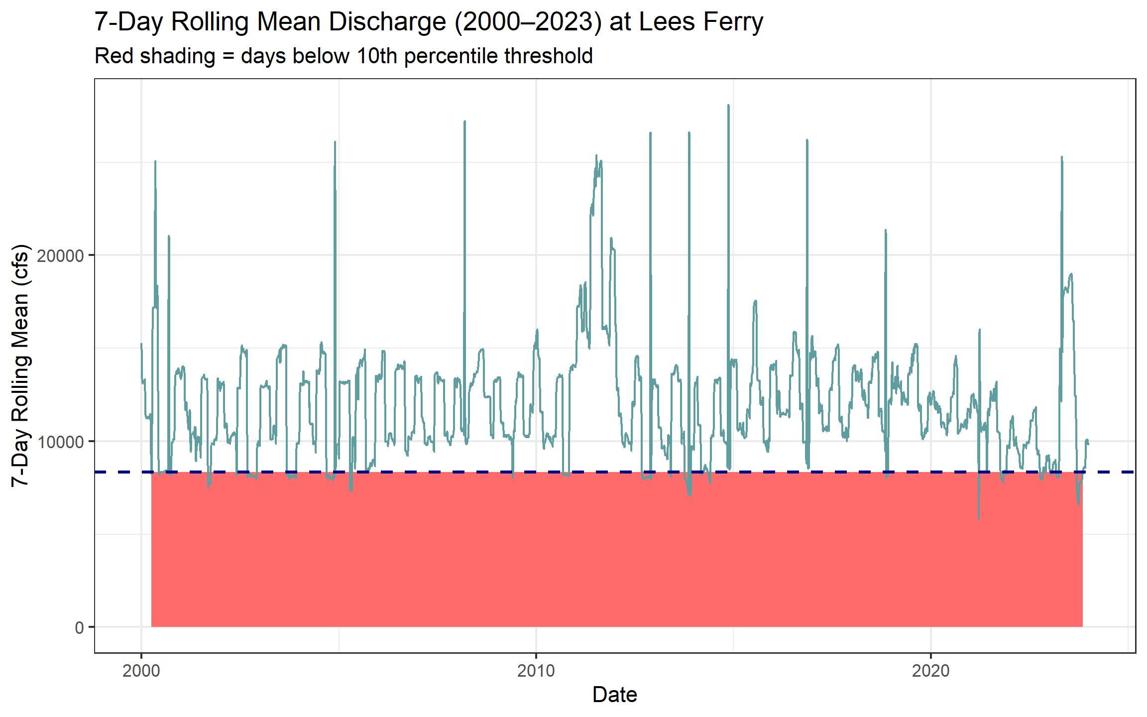

e. How many days per year, on average, did Lees Ferry fall below its low-flow threshold in 2000–2010 vs. 2011–2023? Produce a small summary table and answer in 2–3 sentences: (1) did below-threshold days increase or decrease? (2) Is this a shift in isolated dry years or a persistent baseline change? (3) What does this imply for Compact delivery obligations?

On average below threshold days have increased from 2000-2010 to 2011-2023. It seems like this shows a persistent baseline change. This implies that for meeting the compact requirements for water delivery we need to apply measures that conserves more water, or an amandement that considers future droughts due to climate change.
Congressional Research Service. (2023, May 5). Management of the Colorado River: Water allocations, drought, and the federal role (R45546). https://www.congress.gov/crs_external_products/R/HTML/R45546.html

Tip

n_distinct(year(Date)) counts unique years in a group — useful for computing per-year averages across a multi-year period.

Code

leesferry_below<-leesferry|>
  mutate(periods= if_else(year(Date)<= 2010, "2000–2010", "2011–2023"))|>
  mutate(threshold_limit= if_else(roll7day< threshold, "below", "above"))|>
  group_by(periods)|>
  summarise(total_below= sum(below_threshold_lees, na.rm = TRUE),
            Years= n_distinct(year(Date)),
            mean_days= total_below/ Years)

leesferry_below|>
  flextable()|>
  set_header_labels(total_below= "Total days Below Threshold",
                    mean_days= "Average Days per Year Below Threshold")|>
  set_caption("Average Days per Year Below Threshold in Lees Ferry")|>
  autofit()

periods	Total days Below Threshold	Years	Average Days per Year Below Threshold
2000–2010	399	11	36.27273
2011–2023	358	13	27.53846

Question 5: Annual Water Year Summary

Calendar years are a poor fit for western US hydrology. The water year (October 1 – September 30) captures the full snowmelt cycle: snowpack accumulates through winter, melts in spring, and by September the basin has recharged or drawn down for the year. Water year 2023 = October 1, 2022 through September 30, 2023.

a. Add water_year and month columns to your dataset. The water year is the calendar year of the ending September 30 — months October through December belong to the next water year.

Note

Use if_else() to set water_year for Oct–Dec months.

b. For each gauge and water year, compute: total annual discharge, peak daily discharge, and number of days below the low-flow threshold.

Code

rolling_mean<- rolling_mean|>
  mutate(Month= month(Date),
    water_year= if_else (month(Date)>= 10, year(Date)+1, year(Date) ))

annual_data<- rolling_mean|>
  drop_na(Flow, below_threshold)|>
  group_by(site_no, water_year)|>
  summarise(annual_discharge= sum(Flow),
            peak_daily= max(Flow),
            days_below_thrshold= sum(below_threshold))|>
  arrange(desc(water_year))

c. Plot total annual discharge at Lees Ferry by water year (1980–2023) as a bar chart. Color bars above the long-term median blue and bars below it red. Add a dashed horizontal reference line at the median.

Tip

Hint: compute the long-term median and color bars by whether each year’s total is above or below it; add a dashed horizontal line at the median for reference.

Code

annual_data_lees<- annual_data|>
  filter(site_no== "09380000" & water_year >= 1980, water_year <= 2023)

lees_median<- median(annual_data_lees$annual_discharge)

annual_data_lees<- annual_data_lees|>
  mutate(median = if_else( annual_discharge >= lees_median, "Above Median", "Below Median"))



annual_data_lees|>
  ggplot(aes(water_year, annual_discharge, fill = median))+
  geom_bar(stat= "identity")+
  geom_hline(yintercept = lees_median, color= "darkgreen", linewidth= 1, linetype= "dashed")+
  labs(title= "Total Annual Discharge (1980-2023) at Lees Ferry",
         x= "Water Year",
       y= "Total Annual Discharge")+
  scale_fill_manual(values = c("Above Median"= "lightblue", "Below Median"= "red"))+
  theme_bw()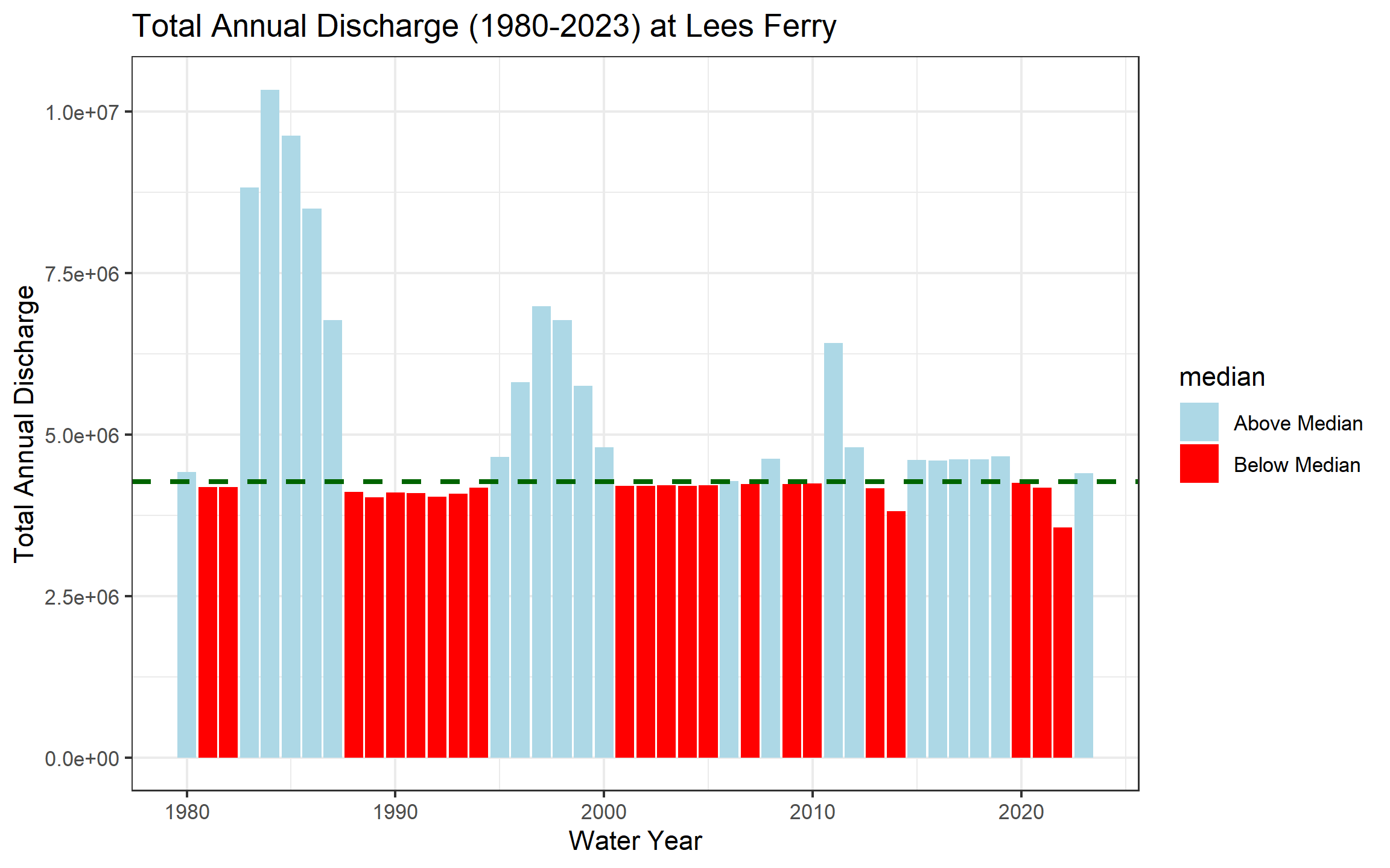

In 2–3 sentences: (1) describe the direction and approximate timing of any structural shift in the record, (2) identify one year that stands out as an exception to the dominant pattern and what you know about its cause, and (3) explain what this pattern means for Compact water accounting.

The plot shows that there is a structural shift to below median discharge around 1983 to 1998, and 1995 to 2000s. It seems that after 2005, we have less high median discharge years comapared to the pattern from previous years. It seems like the years that we have below median discharge in Lees Ferry is decreasing. Although we can not jusdge based on one of the tributaries but if the same pattern exists in other tributaries, this could mean less available water for the Colorado river compact, and could lead to disputes between states. Hogan, D., & Lundquist, J. D. (2024). Recent upper Colorado River streamflow declines driven by loss of spring precipitation. Geophysical Research Letters, 51(16), e2024GL109826.

Question 6: Basin-Wide Trend Analysis

A single gauge tells you about one location. To understand whether drought is consistent across the entire basin — or whether some tributaries are diverging from the main stem — you need to compare all gauges simultaneously on the same scale.

Raw discharge can’t serve this purpose: a large-watershed gauge will always dominate. The solution is a standardized anomaly — each year’s flow expressed as standard deviations above or below the site’s own baseline mean:

\[\text{anomaly} = \frac{\bar{Q}_{year} - \bar{Q}_{baseline}}{\sigma_{baseline}}\]

where baseline = 1980–2010. An anomaly of –2 means “two standard deviations below normal for this gauge” — directly comparable to the same metric at any other gauge.

a. Compute the 1980–2010 baseline mean and SD per gauge. Join those stats back to the full annual data and compute the standardized anomaly for every gauge-year combination.

Tip

Hint: summarize baseline mean and SD per gauge (1980–2010), join those stats to the annual table, and compute the standardized anomaly as (total_flow − baseline_mean)/baseline_sd. This is a join you’ve seen twice now — verify row counts and NAs after the join.

Code

baseline_data<- annual_data|>
  filter(water_year>= 1980, water_year<= 2010)|>
  drop_na(annual_discharge)|>
  group_by(site_no)|>
  summarise(baseline_mean= mean(annual_discharge), baseline_sd= sd(annual_discharge))

baseline_data<- baseline_data|>
  left_join(gauges, by= "site_no")

gauge_anomaly<- annual_data|>
  left_join(baseline_data, by= "site_no")|>
  mutate(standard_anomaly= (annual_discharge- baseline_mean)/ baseline_sd)

nrow(gauge_anomaly) == nrow(annual_data)

[1] TRUE

Code

sum(is.na(gauge_anomaly$standard_anomaly))

[1] 0

b. Visualize as a heatmap: water year on x, gauge name on y, fill = standardized anomaly. Use a diverging color scale centered at zero (blue = above average, red = below average).

Tip

geom_tile() draws one rectangle per gauge-year. For the color scale, use a diverging color scale centered at zero (e.g., RdBu), clamp extreme values with oob = scales::squish, and wrap long gauge names to keep labels readable.

Code

gauge_anomaly|>
  mutate(name= str_wrap(name, width= 20))|>
ggplot(aes(water_year, name, fill= standard_anomaly))+
  geom_tile(color= "white")+
  scale_fill_distiller(palette= "RdYlBu",limits = c(-3, 3), oob = scales::squish, direction= 1) +
  labs(title = "Annual Discharge Anomaly by Gauge Name (1980–2024)",
    x = "Water Year",
    y = "") +
  theme_minimal()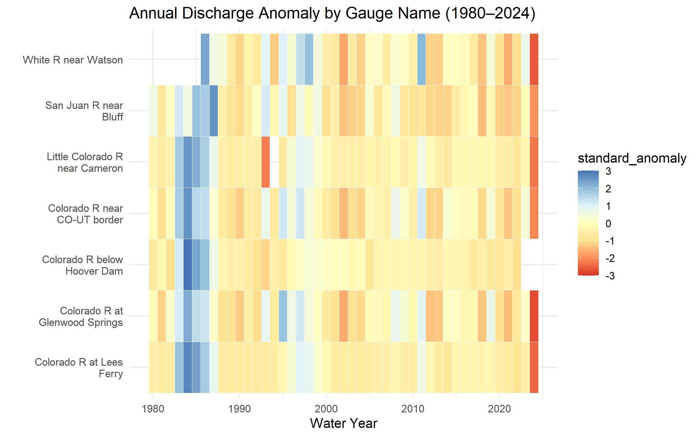

c. In 3–4 sentences: (1) describe whether the post-2000 drought signal appears across all gauges or only some, (2) identify two specific years that appear as basin-wide anomalies — one dry, one wet — and name the climate event that caused each, and (3) explain what simultaneous basin-wide anomalies tell you that a single-gauge record cannot.

The post-2000 drought signal appears across almost all gauges. This shows that there are more drought after 2000s. It seems that 2002 was very dey, and 2011 was weter compared to the trend. The heat map compares all seven gauges across different years and tells us what is happening in the basin overall, and we can see the trend and the relationship. If the heatmap was showing drought only in one of the gauges and others were wet, we would realize that maybe something else is happening in that tributary that is external rather than climate and drought.
Gangopadhyay, S., Woodhouse, C. A., McCabe, G. J., Routson, C. C., & Meko, D. M. (2022). Tree rings reveal unmatched 2nd century drought in the Colorado River Basin. Geophysical Research Letters, 49(11), e2022GL098781. ————————————————————————

Question 7: The Moving Center of Drought

You have been asked to understand how the geographic center of streamflow has shifted over time. If drought has disproportionately reduced flow in the southern tributaries, the flow-weighted center of the basin should drift north — proportionally more flow is coming from northern headwater gauges. In exceptional snowmelt years it should shift back.

We measure this with the flow-weighted mean position: each gauge’s coordinates are weighted by its fraction of total annual basin flow.

\[\bar{X}_{year} = \frac{\sum (lon_i \times Q_i)}{\sum Q_i} \qquad \bar{Y}_{year} = \frac{\sum (lat_i \times Q_i)}{\sum Q_i}\]

a. Join gauge coordinates (dec_lat_va, dec_long_va) from site_meta to your annual summary. Compute the flow-weighted mean latitude and longitude for each water year.

Tip

Hint: join coordinates from site_meta to the annual table, then compute weighted longitude/latitude per year as sum(coord * total_flow) / sum(total_flow). This is your third join — verify row counts, NAs, and spot-check known values.

Note: mapping can use map_data("state"); if map_data() is not available install the maps package (install.packages("maps")) or use ggplot2::map_data("state") which provides equivalent polygons.

Code

annual_coordination<- gauge_anomaly|>
  left_join(site_meta, by= "site_no")

nrow(annual_coordination) == nrow(gauge_anomaly)

[1] TRUE

Code

sum(is.na(annual_coordination$dec_lat_va))

[1] 0

Code

flow_weighted<- annual_coordination|>
  group_by(water_year, site_no)|>
  summarise(weighted_lat=sum(dec_lat_va*annual_discharge)/ sum(annual_discharge),
            weighted_long=sum(dec_long_va*annual_discharge)/sum(annual_discharge))

b. Create a two-panel figure using patchwork:

Left: western US base map with the weighted center plotted as points colored by water year (blue = early, red = recent) and connected by a path through time
Right: line plot of weighted mean latitude over time with a linear trend line

Tip

Hint: draw a western-US polygon basemap and overlay the annual weighted centers as a colored path and points; beside it, plot weighted latitude over time with a linear trend. Use a diverging color gradient for year progression and patchwork to combine panels.

If you haven’t seen patchwork before, it allows you to combine multiple ggplots into a single figure with simple syntax: plot1 + plot2 places them side by side; plot1 / plot2 stacks them vertically assuming the package is loaded.

Code

western_states<- map_data("state")|>
  filter(region %in% c("california", "new mexico", "wyoming","colorado", "utah", "arizona", "nevada"))

plot1<- ggplot() +
  geom_polygon(western_states, mapping= aes(long,lat, group = group), fill= "white", color= "grey") +
  geom_path(flow_weighted, mapping= aes(weighted_long,weighted_lat, color = water_year))+
  geom_point(flow_weighted, mapping= aes(weighted_long, weighted_lat, colour = water_year))+
  scale_color_gradient(low= "blue", high = "red", name= "Water Year")+
  labs(title = "Flow in Western US (1980-2023)",
    x= "longitude",
    y= "latitude")
  
plot2<- ggplot(flow_weighted, mapping= aes(water_year, weighted_lat))+
  geom_line(color= "blue")+
  geom_smooth(method= "lm")+
  geom_point(aes(color=water_year))+
      scale_color_gradient(low= "blue", high = "red", name= "Water Year")+
  scale_y_continuous(limits = c(34,42))+
    labs(title = "Flow weighted Mean over Time",
    x= "Water Year",
    y= "weighted mean latitude")

plot1+plot2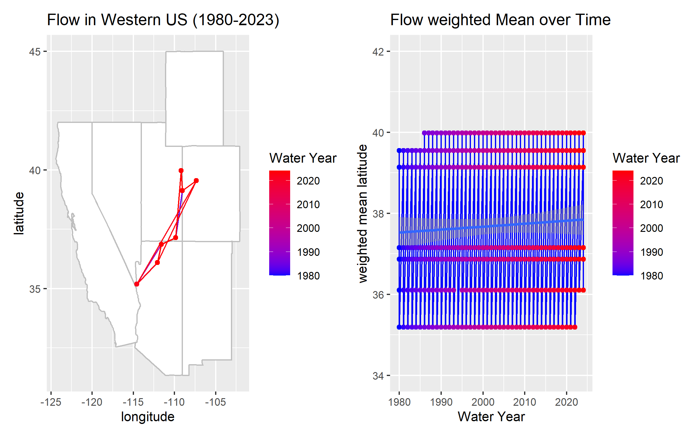

c. Your latitude time series should show two years where the weighted center spikes dramatically northward. Identify those two years and explain: (1) what climate event caused each spike, (2) what they have in common physically, and (3) what the long-term upward trend in weighted latitude suggests about which part of the basin is becoming proportionally more important to total flow — and why that matters for water managers downstream.

The spikes happen in 2011 and 2017. It seams like there has been more flow on those years, which could be a sign of la nina year. They both happen in high elevation. The long-term upward trend in weighted latitude suggests that northern gauges are becoming more important for the flow of the whole basin.
Colorado State University. (2023). Chapter 3: Changes in Colorado’s water. Climate Change in Colorado. https://climatechange.colostate.edu/chapters/3_water.html ————————————————————————

Question 8: Seasonal Regimes and Peak Timing

Annual totals mask important seasonal structure. The Colorado Basin has two distinct runoff pulses: a snowmelt surge in spring (April–June) driven by Rocky Mountain headwater snowpack, and a monsoon pulse in late summer (July–September) driven by convective storms across the Arizona-New Mexico plateau. These seasons respond differently to climate forcing — and under warming, the snowmelt season is arriving earlier.

a. Add a season column using case_when(). Roughly we will define the seasons as follows:

Snowmelt: April–June (months 4–6)
Monsoon: July–September (months 7–9)
Low-flow: October–December (months 10–12)
Winter: January–March (months 1–3)

Make season a factor with levels in hydrological order: Snowmelt, Monsoon, Low-flow, Winter.

Tip

Hint: extract month from Date with lubridate::month(), create season with case_when() mapping month ranges to labels, then convert to a factor with explicit level ordering:

Code

rolling_mean <- rolling_mean|> 
  mutate(
  month = month(Date),
  season = case_when(
    month %in% c(4,5,6) ~ "Snowmelt",
    month %in% c(7,8,9) ~ "Monsoon",
    month %in% c(10,11,12) ~ "Low-flow",
    month %in% c(1,2,3) ~ "Winter"),
  season = factor(season, levels = c('Snowmelt', 'Monsoon', 'Low-flow', 'Winter'))
)

Code

rolling_mean<-rolling_mean|>
  left_join(site_meta, by= "site_no")

rolling_mean<-rolling_mean|>
  mutate(flow_per_sqmi= Flow/drain_area_va)

b. Group by gauge, water year, and season. Summarize total seasonal discharge and normalized runoff per group.

Code

seasonal_flow<-rolling_mean|>
  group_by(site_no, water_year, season)|>
  summarise(total_season_discharge= sum(Flow, na.rm = TRUE), normalized_runoff= sum(flow_per_sqmi, na.rm = TRUE))

c. For each gauge and water year, identify the date of peak 7-day mean flow and convert it to day-of-year. Plot peak day-of-year vs. water year for Lees Ferry with a linear trend line.

Tip

slice_max(roll7, n = 1, with_ties = FALSE) inside a group_by(site_no, water_year) block selects the single highest 7-day mean row per gauge per year. Then lubridate::yday(Date) converts to day-of-year (1–365).

Code

peak_day_flow<- rolling_mean|>
  drop_na(Flow, roll7day)|>
  group_by(site_no, water_year)|>
  slice_max(roll7day, n = 1, with_ties = FALSE)|>
  ungroup()|>
  mutate(peak_day= lubridate::yday(Date))

peak_day_flow|>
  filter(site_no == "09380000")|>
  ggplot(aes(water_year, peak_day))+
  geom_point(aes(color = water_year))+
  geom_smooth(method = "lm", se = TRUE, color= "red")+
  labs(title = "Peak 7-Day Mean Flow vs Water Year
       for Lees Ferry",
       x= "Water Year",
       y= "Peak Day")+
  theme_bw()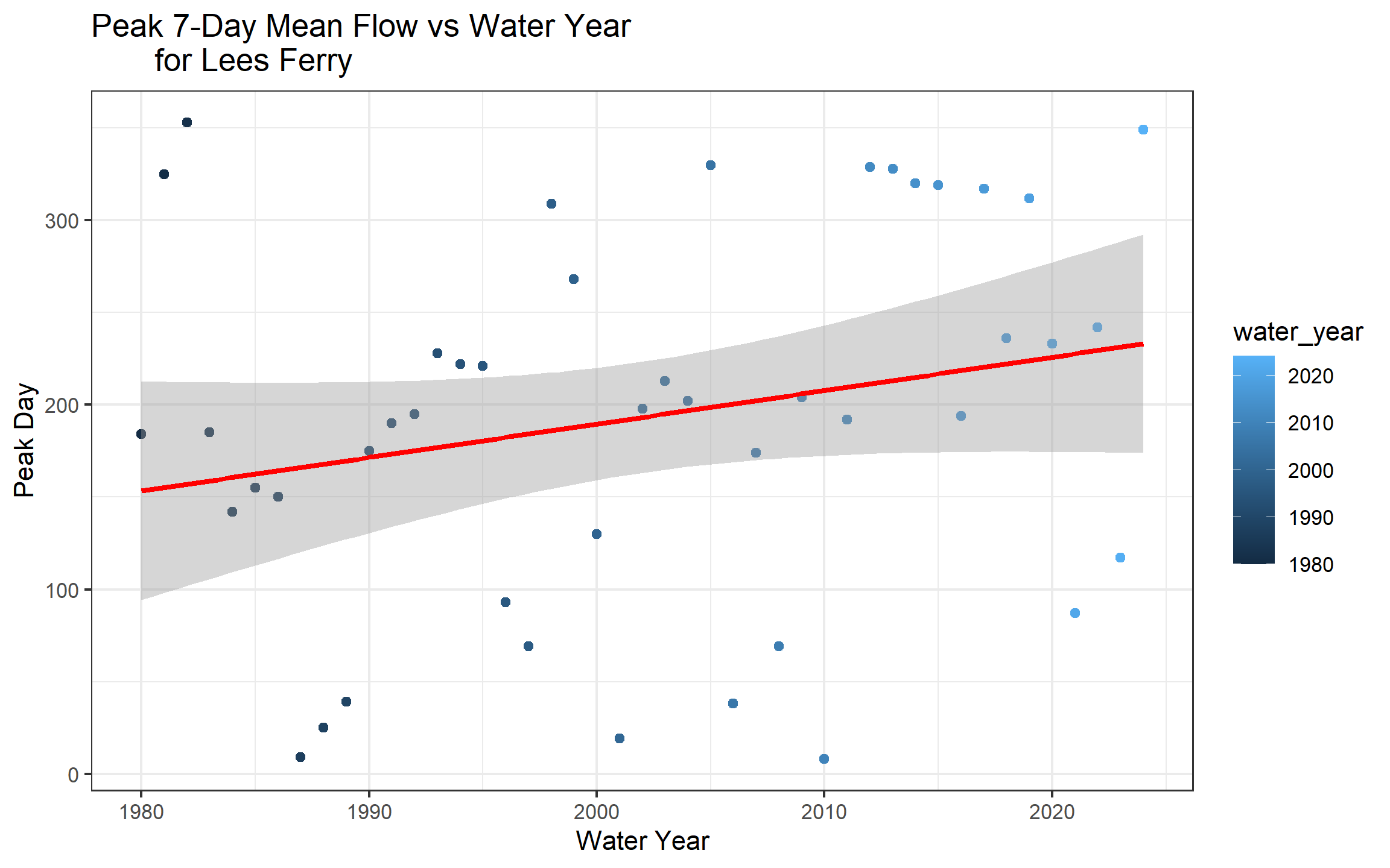

d. In 2–3 sentences: (1) describe the direction and magnitude of the peak timing trend, (2) is it statistically visible or buried in noise? (3) What would a two-week earlier peak timing mean operationally for reservoir managers trying to capture spring runoff before it passes downstream?

The trend shows that the peak timing is happening earlier than before, and the overall trend is increasing. The trend line shows it specifically, but I think the trend is clear statistically, however a test would help us see it clearer. It means they have a short time between snowmelt and peak flow and they have less time to capture the runoff before it passes downstream.
Christensen, N. S., Wood, A. W., Voisin, N., Lettenmaier, D. P., & Palmer, R. N. (2004). The effects of climate change on the hydrology and water resources of the Colorado River basin. Climatic change, 62(1), 337-363.
Wheeler, K., Kuhn, E., Bruckerhoff, L., Udall, B., Wang, J., Gilbert, L., … & Schmidt, J. C. (2021). Alternative management paradigms for the future of the Colorado and Green Rivers. The Future of the Colorado River Project, White Paper No. 6. Logan, UT: Utah State University, Quinney College of Natural Resources Center for Colorado River Studies. 132 p. ————————————————————————

Question 9: Predicting Lees Ferry from Upstream Conditions

Lees Ferry is the Compact’s accounting point — the location where upper basin states must deliver flow to lower basin states. Predicting annual discharge at Lees Ferry from upstream conditions has direct operational value: managers can begin planning deliveries months before the water arrives.

We’ll build a simple but physically grounded model: can Glenwood Springs (an upper Rocky Mountain gauge) predict Lees Ferry annual flow, and, does that relationship change by season?

Data Preparation

a. Build your model dataset through four sequential operations:

Filter annual to Lees Ferry; rename total_flow to lees_flow
Join annual Glenwood Springs flow (site 09085000); rename to glenwood_flow
Join the dominant season at Lees Ferry per water year, the season with the highest total discharge
Log-transform both flow variables

Tip

The dominant season: within each water year, which season (Snowmelt, Monsoon, Low-flow, Winter) carried the most flow at Lees Ferry? Filter seasonal summaries to Lees Ferry, then group_by(water_year) |> slice_max(total_flow, n = 1) to select one season per year.

Then join that back to your Lees Ferry & Glenwood annual table by water_year.

This is your fourth join. Always verify: the final dataset should have ~44 rows (one per water year, 1980–2023), zero NAs in flow columns, and log-transformed values should be positive.

Code

#1
lees_annual <- annual_data|>
  filter(site_no == "09380000")|>
  rename(lees_flow = annual_discharge)
# I already filtered this above it is called annual_data_lees but in here it is not asking us to filter to up to 2023 so i can not use the same dataset

#2
glenwood_annual<- annual_data|>
  filter(site_no == "09085000")|>
  rename(glenwood_flow = annual_discharge) 

lees_model_data<- lees_annual|>
  left_join(glenwood_annual, by = "water_year")

#3
dominant_season<- seasonal_flow|>
  filter(site_no == "09380000")|>
  group_by(water_year)|>
  slice_max(total_season_discharge, n = 1)|>
  ungroup()|>
  select(water_year, season)

lees_model_data<- lees_model_data|>
  left_join(dominant_season, by = "water_year")

#4
lees_model_data<- lees_model_data|>
  mutate(log_lees= log(lees_flow),
         log_glenwood =log(glenwood_flow))

nrow(lees_model_data)

[1] 45

Code

sum(is.na(lees_model_data$log_lees))

[1] 0

Code

sum(is.na(lees_model_data$log_glenwood))

[1] 0

Code

sum(is.na(lees_model_data$season))

[1] 0

Model Building

b. Fit a linear model predicting log_lees from log_glenwood, season, and their interaction, If you haven’t seen linear modeling in R, we will cover it in more detail latter in this course, but, the syntax is straightforward: lm(response ~ predictor1 * predictor2, data = mydata) fits a model with main effects and an interaction term. The interaction (*) allows the relationship between Glenwood and Lees to differ by season while a model without interaction (lm(log_lees ~ log_glenwood + season)) would assume the same Glenwood-Lees relationship in every season.

Code

mod <- lm(log_lees ~ log_glenwood * season, data = lees_model_data)
summary(mod)


Call:
lm(formula = log_lees ~ log_glenwood * season, data = lees_model_data)

Residuals:
     Min       1Q   Median       3Q      Max 
-0.27318 -0.06674 -0.01845  0.03116  0.56633 

Coefficients:
                            Estimate Std. Error t value Pr(>|t|)    
(Intercept)                  -8.1111     5.2755  -1.538 0.132679    
log_glenwood                  1.7973     0.3965   4.533  5.9e-05 ***
seasonMonsoon                20.1902     5.4095   3.732 0.000636 ***
seasonLow-flow               12.1775     5.3668   2.269 0.029188 *  
seasonWinter                 23.0070     8.4608   2.719 0.009904 ** 
log_glenwood:seasonMonsoon   -1.5459     0.4072  -3.796 0.000529 ***
log_glenwood:seasonLow-flow  -0.9088     0.4042  -2.249 0.030584 *  
log_glenwood:seasonWinter    -1.7699     0.6535  -2.708 0.010181 *  
---
Signif. codes:  0 '***' 0.001 '**' 0.01 '*' 0.05 '.' 0.1 ' ' 1

Residual standard error: 0.1535 on 37 degrees of freedom
Multiple R-squared:  0.8553,    Adjusted R-squared:  0.8279 
F-statistic: 31.25 on 7 and 37 DF,  p-value: 1.127e-13

c. In 3–4 sentences: (1) report the R² and state whether the overall model is statistically significant, (2) interpret the log_glenwood coefficient as an elasticity — what does it mean physically that the coefficient is greater than 1? (3) describe what the significant negative interaction terms tell you about the upstream-downstream relationship outside of Snowmelt season.

Tip

In a log-log model, the coefficient on log_glenwood is an elasticity: a coefficient of 1.8 means a 1% increase in Glenwood Springs flow is associated with a 1.8% increase at Lees Ferry. This super-linear amplification makes physical sense — flow accumulates from tributaries between the two gauges, so an above-average headwater year compounds as it moves downstream.

R^2= 0.855, adjusted R^2= 0.828. This means that the model explains 85.5 of the variance in annual flow in Lees Ferry. The log_glenwood coef equals to 1.797 and it means that 1% increase in flow in Glenwood is associated with 1.797% increase at Lees Ferry. The significant negative interaction terms for Monsoon (−1.55), Low-flow (−0.91), and Winter (−1.77) show that the upstream downstream relationship is not the same during the Monsoon and winter seasons. and Lees ferry and Glenwood are independent from each other.
Grant, C. D. (2024). Quantifying the Price Elasticity of Water Demand in Cheyenne, WY: Implications for Drought Management and Policy in the Colorado River Basin. University of Wyoming. ————————————————————————

Question 10: Model Evaluation

A model that fits well on average can still fail in predictable ways. Two core assumptions of linear regression are: predictions should be unbiased across the full range of fitted values, and residuals should be approximately normally distributed. Let’s check both — and look for the outlier year that the model cannot predict.

a. Use broom::augment() to produce a tidy data frame of predictions and residuals alongside the original data:

Code

aug <- augment(mod, data = lees_model_data)

Introducing broom

broom converts messy R model objects into tidy, pipeable data frames:

augment(mod) — adds .fitted (predictions) and .resid (residuals) to your data
glance(mod) — one-row summary of model fit: R², AIC, p-value
tidy(mod) — one-row-per-coefficient table with estimates and p-values

Together these make model results as pipeable as any other data frame — straight into ggplot or flextable.

b. Create a predicted vs. actual scatter plot. Add a dashed 1:1 reference line (perfect prediction). Color points by season. Identify any point that sits noticeably off the line.

Tip

geom_abline(slope = 1, intercept = 0, linetype = "dashed") draws the 1:1 line. Points above it = underpredicted (actual > predicted); points below = overpredicted.

Code

aug|>
  ggplot(aes(x = .fitted, log_lees, colour= season))+
  geom_point()+
  geom_abline(slope = 1, intercept = 0,
              linetype = "dashed")+
  geom_text(data= aug |> filter(abs(.resid) > 0.2),
    aes(label = water_year)) +
  labs(title = "Predicted vs. Actual Lees Ferry Flow",
    x = "Predicted",
    y= "Actual")+
  theme_minimal()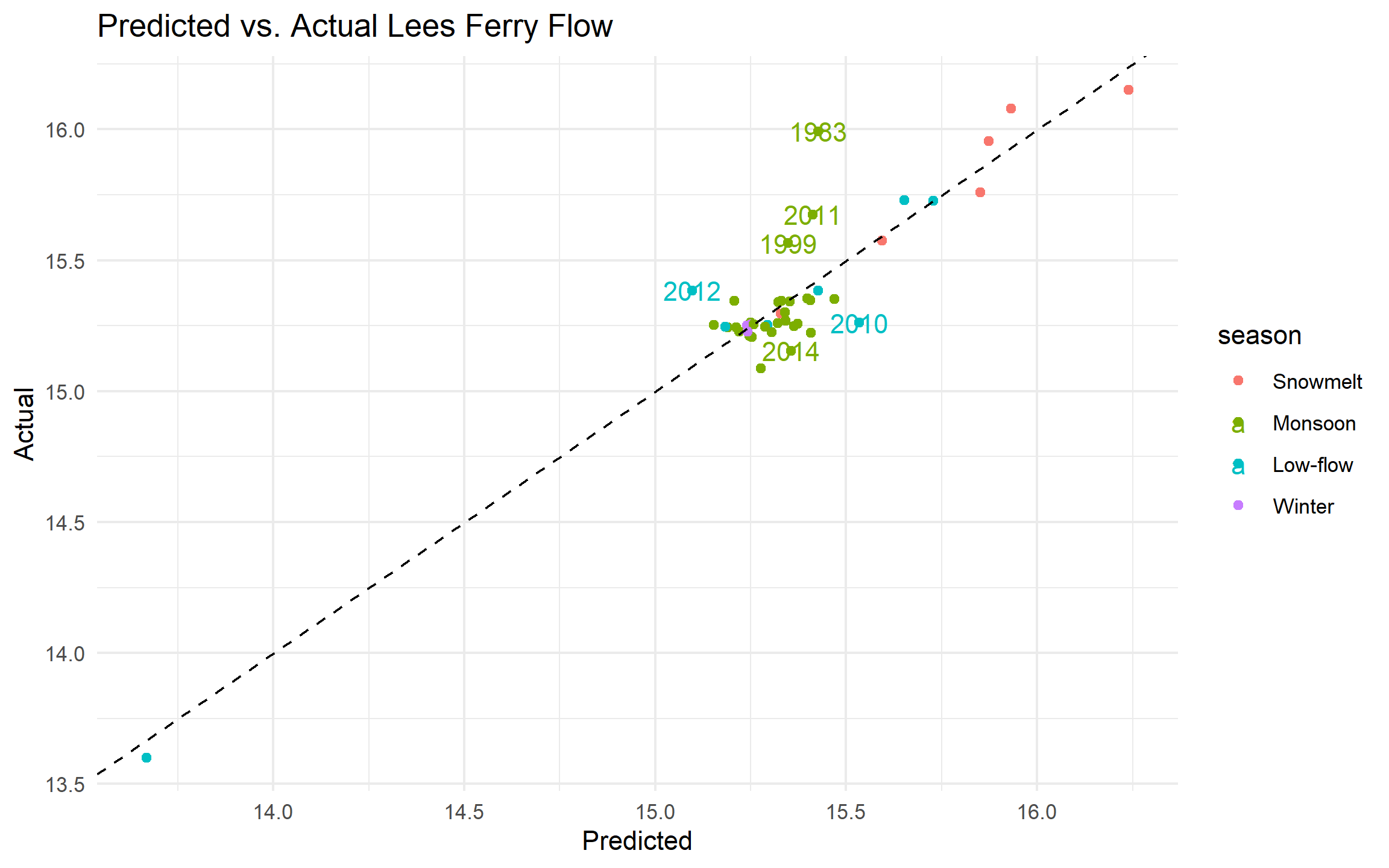

c. Plot a histogram of the residuals with a vertical dashed line at zero.

Code

aug|>
ggplot(aes(x = .resid))+
  geom_histogram(fill = "pink") +
  geom_vline(xintercept = 0,linetype = "dashed", linewidth=0.6) +
  labs(title= "Histogram for Lees Ferry Flow Model",
    x= "Residual")+
  theme_minimal()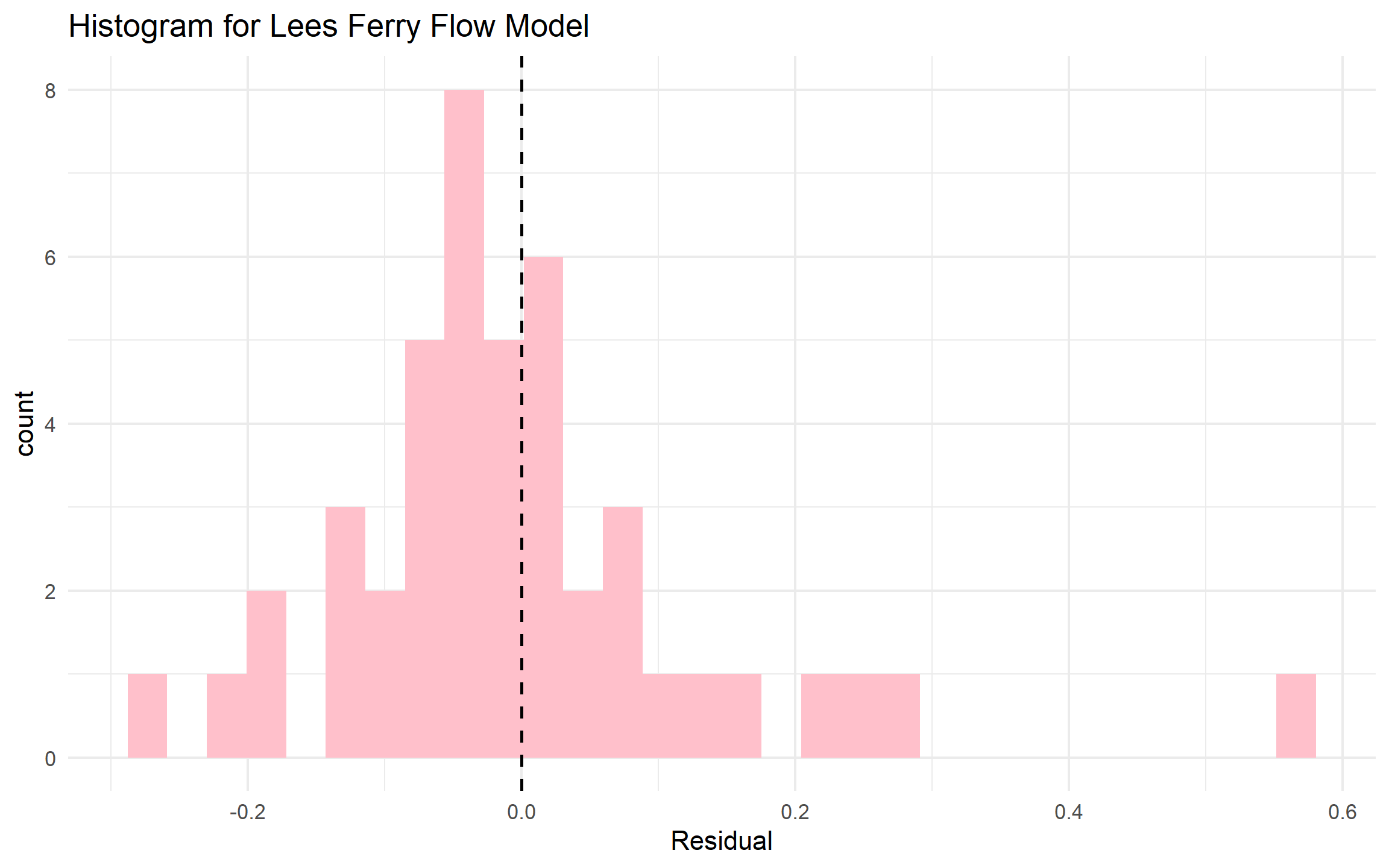

d. In 3–4 sentences: (1) identify the outlier water year visible in your scatter plot. Which year is it and why did the model fail to predict it? (2) Do the residuals appear approximately normal, or is there a tail that concerns you? (3) Name two additional predictors that would most improve this model and explain the physical mechanism behind each.

There are several outliers including the year 1983, 2011, 2012. The model fail to predict it because the difference in the flow capture that year. The residuals appear normal with outlier on the right tail. I think two predictors could be snowpack, that helps measure the water from melting, and climate drivers such as el nino la nina as they can cause above average measures for different years.
Serreze, M. C., Clark, M. P., Armstrong, R. L., McGinnis, D. A., & Pulwarty, R. S. (1999). Characteristics of the western United States snowpack from snowpack telemetry (SNOTEL) data. Water Resources Research, 35(7), 2145-2160. ————————————————————————

Going Further (ungraded)

The model in Q9 predicts Lees Ferry from a single upstream gauge. dataRetrieval gives you access to hundreds more across the basin. Could a multi-gauge ensemble prediction outperform the single-gauge model? Could peak flows in March predict the following June’s flow at Lees Ferry months before snowmelt begins?

These are real operational forecasting questions that USBR and state water agencies work on every year. The data is already in your hands to try!

Summary

In this lab you built a complete analytical pipeline for one of the most consequential river systems in North America:

Retrieved 44 years of daily streamflow directly from the USGS NWIS API using dataRetrieval
Joined gauge metadata using relational keys — and verified every join
Normalized by drainage area to enable fair comparisons across the basin
Detected low-flow threshold exceedances using rolling statistics for operational drought monitoring
Aggregated by water year and season — the natural temporal units of western hydrology
Visualized basin-wide trends with a standardized anomaly heatmap and a flow-weighted spatial center analysis
Modeled the upstream-downstream relationship at the Compact’s accounting point
Evaluated model assumptions and identified the outlier year the model couldn’t predict

Every tool — dplyr, ggplot2, zoo, patchwork, broom, flextable — recurs in work you will inevitabbly do. The key is that the workflow is always the same: get → tidy → explore → model → communicate.

Rubric

Question	Topic	Points
Q1	Daily conditions report	10
Q2	Basin metadata join	10
Q3	Per-unit-area normalization	10
Q4	Low-flow threshold monitoring	20
Q5	Annual water year summary	10
Q6	Basin-wide trend analysis	15
Q7	Moving center of drought	15
Q8	Seasonal regimes + peak timing	15
Q9	Predictive model	15
Q10	Model evaluation	10
Well-structured, legible Qmd	—	10
Deployed as a webpage	—	10
Total		150

Grading key (brief): - Correctness (primary): calculations, joins, and checks — e.g., Q2 join verification and Q4 rolling mean logic. - Reproducibility: code runs end-to-end, used parameter objects (my.date), and included any small checks or assertions. - Clarity & Presentation: readable code, labeled tables/plots, captions for flextable outputs, and a clear 1-paragraph interpretation.

Submission

Render: quarto render lab-01.qmd
Push: git add -A && git commit -m "lab 1 complete" && git push
Activate GitHub Pages: GitHub → Settings → Pages → Deploy from branch → main
Submit your live URL to Canvas: https://USERNAME.github.io/csu-523c/lab-01.html

Add this project to your personal website with a brief description — it counts toward end-of-semester extra credit.